Architecture
sparsegrad performs forward mode automatic differentiation on vector valued function.
sparsegrad forward value is a pair  where y is referred to as
 value and the Jacobian  is referred to as
 dvalue.
During the evaluation, sparsegrad values are propagated in place of standard numpy arrays. This simple approach gives good result when only first order derivative is required. Most importantly, it does not involve solving graph coloring problem on the whole computation graph. For large problems, storing complete computation graph is very expensive.
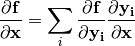
When a mathematical function 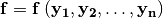 is evaluated, the derivatives are propagated using the chain rule
Support for numpy
To support numpy functions, broadcasting must be included. In the discussion below, scalars are treated as one element vectors.
Application of a numpy function involves implicit broadcasting from vector  , with its proper shape, to vector
  , with shape of
  if both shapes are not the same. This can be denoted by multiplication by matrix
  . The result of function evaluation is then

and the derivative is
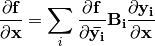
The Jacobian of numpy function application is a diagonal matrix. If  is a
is a numpy elementwise derivative of with respect of to , then
Optimizations
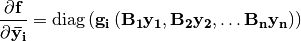
As a major optimization, the Jacobian matrices are stored as a product of scalar  , diagonal matrix
  and a general sparse matrix
  :
:
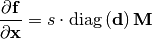
The general parts are constant shared objects. If not specified, the diagonal parts and the general parts are assumed to be identity.
The factored matrix is referred to as sdcsr in sparsegrad code. It allows to peform the most common operations with rebuilding the general matrix part:
![\left[ s_1 \cdot \mathrm{diag} \left( \mathbf{d_1} \right) \mathbf{M} \right] +
\left[ s_2 \cdot \mathrm{diag} \left( \mathbf{d_2} \right) \mathbf{M} \right] =
\mathrm{diag} \left ( s_1 \cdot \mathbf{d_1} + s_2 \cdot \mathbf{d_2} \right ) \mathbf{M}](_images/math/0308d9eae721def2f572481fb545d2168e3ee64e.png)
![\alpha \cdot \mathrm{diag} \left( \mathbf{x} \right)
\left[ s \cdot \mathrm{diag} \left( \mathbf{d} \right) \mathbf{M} \right] =
\left( \alpha s \right) \cdot
\mathrm{diag} \left( \mathbf{x} \circ \mathbf{d} \right)
\mathbf{M}](_images/math/1b12a5caff9cc2625fd2b9fdcdafa54a26e74561.png)
with  denoting elementwise multiplication.
Backward mode
Backward mode is currently not implemented because of prohibitive memory requirements for large calculations. In backward mode, each intermediate value has to accessed twice: during the forward evaluation of function value, and during backward evaluation of derivative. The memory requirements to store intermediate values are prohibitive for functions with large number of outputs, and grows linearly with the number of steps in computation.